

Do you often need to work with numbers in Excel that include leading zeros, like 00123, or very large numbers, such as 1234 5678 9087 6543? These could be social security numbers, phone numbers, credit card numbers, product codes, report numbers, or postal codes. Excel, by default, automatically removes leading zeros and converts large numbers into scientific notation, like 1.23E+15, to make calculations easier.
However, this automatic formatting can be problematic when you need to preserve the original format of these numbers, as it changes how they appear and can cause issues when you’re managing data that should remain in a specific format.For example, if you’re entering a product code like 00123, Excel will automatically drop the zeros and display it as 123. Similarly, if you input a large number such as a credit card number, Excel might change it to scientific notation, making it difficult to read and work with. This is because Excel is designed to treat numbers as data for calculations, so it applies formatting rules that prioritize numeric operations over maintaining the appearance of the numbers.
This guide will show you how to keep your data in its original format, ensuring that Excel treats these numbers as text rather than numeric data. By learning how to properly format your cells, you can prevent Excel from altering your data and keep your information accurate and easy to manage. This is essential for working with any data where the specific format is important, such as in the examples mentioned above.
“Preserve Number Formats When Importing Text Data in Excel”
To preserve number formats when importing text data into Excel and convert numbers to text, follow these steps:
1. Open Excel and Start Import Process:
– Launch Excel and go to the “File” tab.
– Select “Open” and choose the text file you want to import. Alternatively, you can start by going to the “Data” tab and selecting “From Text/CSV” to import data directly.
2. Choose the Text File:
– Navigate to the location of your text file, select it, and click “Import” or “Open” to start the import process.
3. Select Data Type in Text Import Wizard:
– If the Text Import Wizard appears, choose the “Delimited” option if your data is separated by commas, tabs, or other characters, or choose “Fixed width” if your data has aligned columns with spaces between them. Click “Next” to proceed.
4. Specify Delimiters or Column Breaks:
– If you selected “Delimited,” choose the character that separates your data (e.g., comma, tab, semicolon) and click “Next.”
– For “Fixed width,” click to set the column breaks where the data should be separated, then click “Next.”
5. Set Column Data Format:
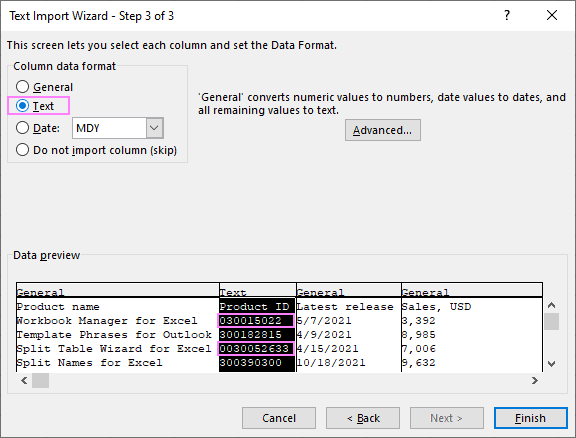
– In the next step, select each column in the data preview window and choose “Text” as the Column Data Format. This will ensure that Excel treats all entries in that column as text, preserving leading zeros and preventing large numbers from converting to scientific notation.
6. Complete the Import:
– Once you’ve set the format for all relevant columns, click “Finish” to complete the import. Excel will now import your data with numbers preserved as text.
7. Save Your Workbook:
– After the data is successfully imported, save your workbook to retain the formatting by clicking “File” and then “Save As.” Choose your desired location and file format.
“Using Custom Formats in Excel to Retain Leading Zeros”
To retain leading zeros in Excel using a custom format, follow these steps:
1. Highlight the Cells:
– Start by selecting the cells that contain the numbers where you want to keep the leading zeros. You can select individual cells, a range of cells, or an entire column as needed.
2. Access the Format Cells Dialog Box:
– Right-click on the highlighted cells and choose “Format Cells” from the context menu. Alternatively, press `Ctrl + 1` on your keyboard to directly open the Format Cells dialog box.
3. Navigate to the Number Tab:
– In the Format Cells dialog, go to the “Number” tab, where various number formatting options are available.
4. Choose the Custom Category:
– In the “Category” list on the left side, scroll down and select “Custom.” This option lets you create a specific format to maintain the leading zeros.
5. Input a Custom Format:
– In the “Type” field, enter a format code that specifies the total number of digits, including leading zeros.
For example: – Enter `00000` for numbers with five digits (e.g., 00123).
– Enter `0000000000` for numbers with ten digits (e.g., 0012345678).
– The number of zeros in the code represents the total length of the number, with leading zeros added to fill the required length.
6. Apply the Custom Format:
– After typing your custom format, click “OK” to apply it. The selected cells will now display numbers with leading zeros according to the custom format you’ve specified.
7. Review the Changes:
– Check your data to confirm that the numbers are displayed correctly with the desired number of leading zeros. This formatting will remain consistent, even if you edit the data or input new numbers.
8. Save the File:
– To keep this custom format intact, save your Excel workbook by clicking “File” and then “Save As.” Select your preferred file format and save location.
Following these steps will ensure that leading zeros are preserved in your Excel data, which is particularly important for product codes, IDs, or any other numerical information where leading zeros are significant.
“Mastering Text Formatting with the TEXT Function”
How to Use the TEXT Function for Formatting:
1. Get to Know the TEXT Function:
– The function’s basic formula is: `=TEXT(value, format_code)`
– Value: The data (like a number or date) you want to format.
– Format_code: The specific code that tells Excel how to display the value.
2. Learn Common Formatting Codes:
– Explore basic codes such as `”0.00″` for decimals, `”mm/dd/yyyy”` for dates, and `”###,###”` for adding commas.
– Try out these codes to see how they change the data’s appearance.
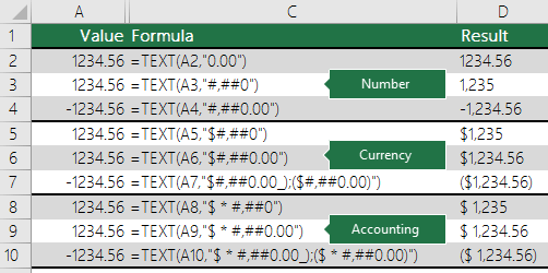
3. Format Numbers with the TEXT Function:
– Example: Turn a number into currency.
– Formula: `=TEXT(1234.567, “$0.00”)`
– Result: `$1234.57`.
4. Format Dates Using TEXT:
– Example: Display the current date in a different format.
– Formula: `=TEXT(TODAY(), “dddd, mmmm dd, yyyy”)`
– Result: “Sunday, August 25, 2024”.
5. Combine TEXT with Other Functions:
– Example: Create a custom message by combining TEXT with `&`.
– Formula: `”Your total is ” & TEXT(1234.567, “$0.00”)`
– Result: “Your total is $1234.57”.
6. Practice and Experiment:
– Experiment with different formats, such as percentages or times.
– The more you practice, the more comfortable you’ll get with using the TEXT function.
7. Double-Check Your Work:
– Review your formulas to ensure they display data the way you want.
– Adjust the format codes as needed for the desired result.
By following these steps, you can easily format your data using the TEXT function.
Conclusion
Keeping leading zeroes in Excel is important for maintaining the accuracy of certain data types, like zip codes, phone numbers, or other identifiers that start with zero. Excel, by default, treats numbers without considering leading zeroes, which can cause them to be removed automatically. To prevent this and ensure your data displays correctly, you can use a few simple methods.
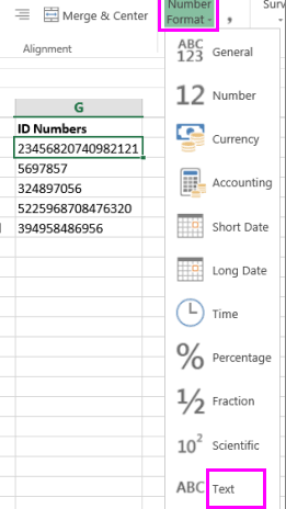
First, you can format the cells as “Text” before entering the data. This tells Excel to treat the information as plain text rather than a number, so the leading zeroes are preserved.
Another method is to use custom number formatting. By applying a format that includes the number of digits you need, Excel will automatically add leading zeroes where necessary. For example, if you want a five-digit code, you can use a format like `”00000″` to make sure all entries display with five digits, even if they start with zeroes.
Lastly, you can use the `TEXT` function to format numbers with leading zeroes dynamically. This is especially useful when working with formulas or if you need to ensure consistent formatting across multiple cells.
These simple techniques help maintain the integrity of your data and ensure it displays as intended.