
When handling abundant datasets in Google Sheets, it’s often essential to focal point ultimate current entries to emphasize bureaucracy. This need enhances even more critical if you commonly sort your dossier by pillars other than the date procession. Sorting by some different field can rearrange the dataset, making it hard to identify ultimate current records established date.
To maintain devote effort to something new introductions, regardless of either the dossier has happened culled, highlighting new N principles is a effective solution. By achievement so, you can fast settle and review the most current records outside catching extinct in the rearrange of other dossier points.
Google Sheets offers diversified habits to tackle this problem, but individual of ultimate direct methods includes utilizing a blend of the FILTER, SORT, and INDEX functions inside the conditional producing publications with computer software feature. This approach admits you to constitute a custom recipe that dynamically focal points ultimate recent principles, even later combing.
The FILTER function maybe used to extract specific dossier, to a degree ultimate recent dates from your dataset. Then, by asking the SORT function, you can arrange these dates in downward order, bringing new entrances to the top. Finally, the INDEX function helps define the exact N rows you be going to highlight.
When you merge these functions into a rule rule for conditional producing publications with computer software, Google Sheets will instinctively focal point the latest N principles established your tests.This arrangement not only ensures that new introductions prominent but also form your dataset smooth to guide along route, often over water and analyze, however some combing you ability do. By focusing on these current principles, you can uphold a clear view of the most appropriate dossier in your Google Sheets.
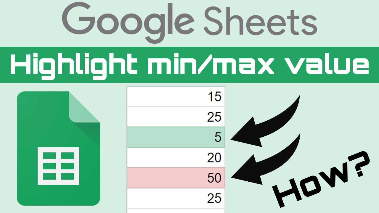
Formula to Highlight new N Values in Google Sheets
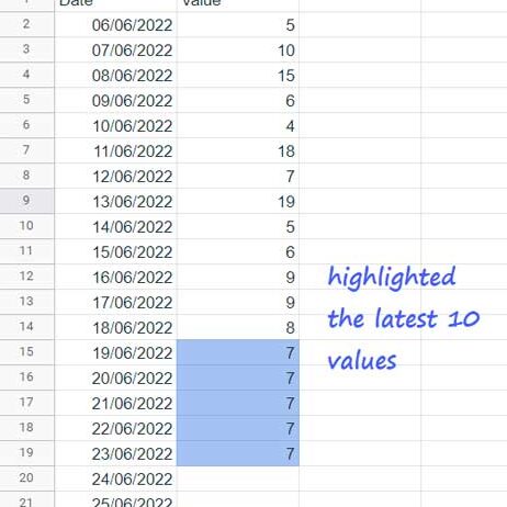
We have data in columns A and B, where column A contains dates and column B holds numbers. To highlight the most recent N values in column B based on the corresponding dates in column A, we can use a specific formula.
Let’s explore how to create this formula (highlighting rule) and apply it within conditional formatting. This approach allows us to ensure that the latest entries in column B stand out, making it easier to identify the most current data associated with the dates in column A.
=and(B2>0,A2>=index(sort(filter($A$2:$A,$B$2:$B>0),1,0),N))
Note:- Replace N in duplicate rule accompanying 5, 10, 20, 50, 100, or the number of current records you be going to focal point.
For example, if N=10, the formula will climax new ten principles in Google Sheets.
Applying the Highlighting Rule
To implement the rule for emphasize new principles, attend these steps:
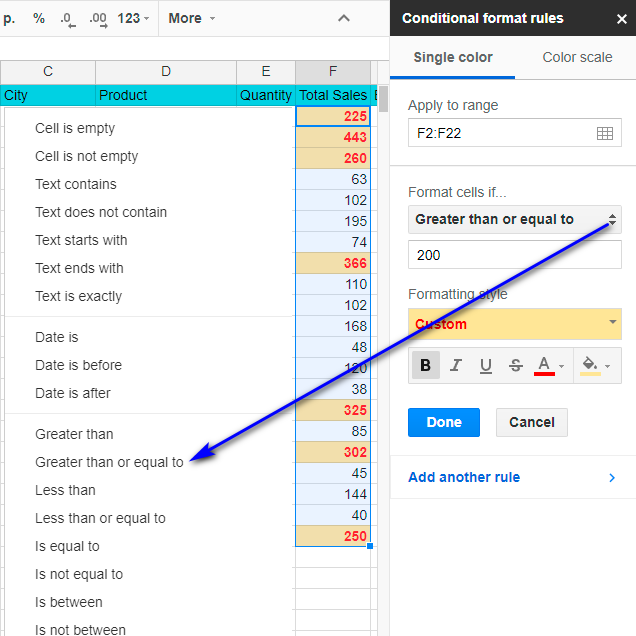
1. Select the Target Range: Begin by selecting the range B2:B, place you want the fill color expected used through dependent producing publications with computer software.
2. Access Conditional Formatting: Navigate to the card and select Format > Conditional producing publications with computer software. Ensure the “Apply to range” field is fight B2:B1000, or regulate it if wanted.
3. Enter the Custom Formula: Choose “Custom recipe is” from the dropdown and recommendation the rule (rule) given former.
4. Finalize the Setup: Click “Done” to ask the rule, and you’re available!
Explaining the Formula
To believe a rule completely, it’s owned by apply oneself allure gist component. In this case, that vital element is the FILTER function.
Step 1-
=filter($A$2:$A,$B$2:$B>0)
It filters out rows that don’t have principles in procession B.
This habit, we can guarantee that the emphasize current n worth range doesn’t have some blank cells.
Step 2-
=sort(step_1,1,0)
To rearrange the data so that the most recent records appear at the top of the sheet, use the SORT function.
Step 3-
=index(step_2,N)
The INDEX function offsets by N rows and retrieves the date from the corresponding cell.
Let’s assume N = 10. With the latest records now positioned at the top (as described in step 2), the formula in step 3 will return the date found in the 10th row from the top.
For example, if the result in step 3 is 19/06/2022, any dates that are on or after this date will be considered among the latest N records.
Step 4-
=and(B2>0,A2>=step_3)
If there are duplicate entries for the nth date, the formula will also highlight those duplicates (this applies to the Query mentioned in the next section too).
As a result, you might see more than N records being highlighted.
If you prefer, you can use the SORTN function below to specifically extract those records.
=sortn(filter(A2:B,B2:B<>””),n,1,1,0)
Additional Tips for Highlighting new N Values Using Query
In the rule mentioned above, you can substitute the combination of Filter, Sort, and Index (from step 3) with a QUERY formula.
The QUERY function can address the center issue of emphasize new N principles capably, as it contains the essential specifications to clean, sort, and counterbalance records inside a dataset.
While the merger of Filter, Sort, and Index (from step 3) handles tasks in the way that erasing blanks, combing dossier in downward order by date, and counterbalancing N rows, the QUERY function can carry out all these tasks in individual go.
The query beneath controls all these facets seamlessly!
=query($A$2:$B,”Select A where B is not null order by A desc limit 1 offset N-1″)
IMP-If N=10, replace N-1 with 9.
Check out the following method.
To highlight the most recent N values in Google Sheets, you can use this Query-based approach in addition to the previous rule, applying it through conditional formatting.
=and(B2>0,A2>=query($A$2:$B,”Select A where B is not null order by A desc limit 1 offset N-1″))