
The COUNT function in Google Sheets allows you to tally all cells with numbers within a specific data range. In other words, COUNT deals with numeric values or those that are stored as numbers in Google Sheets.
The syntax of Google Sheets COUNT and its arguments is as follows:
COUNT(value1, [value2,…])
- Value1 (required) — stands for a value or a range to count within.
- Value2, value3, etc. (optional) — additional values that are going to be covered as well.
What can you use as an argument? The value itself, cell reference, range of cells, named range.
What values can you count? Numbers, dates, formulas, logical expressions (TRUE/FALSE).
If you change the content of any cell from within the counted range, the function will automatically recalculate the result.
If multiple cells contain the same value, COUNT in Google Sheets will return the number of all its instances in those cells.
So to be more precise, the function counts the number of times numeric values appear within the range rather than checks if any of the values are unique.
Google Sheets COUNTA works in a similar way and its syntax is alike:
COUNTA(value1, [value2,…])
- Value (required) — the values you need to count.
- Value2, value3, etc. (optional) — any other additional values to count.
What’s the difference between COUNT and COUNTA? In the values they process.
As you can see, the main difference between the functions lies in the ability of COUNTA to process those values that Google Sheets stores as text. Both functions ignore completely empty cells.
How To Use Google Sheets COUNT and COUNTA functions – With Examples
Let’s take a closer look at how the COUNT function is used in a Google spreadsheet and how you can benefit from using it in Sheets.
Suppose you have a list of students’ grades. Here are the ways COUNT can help:
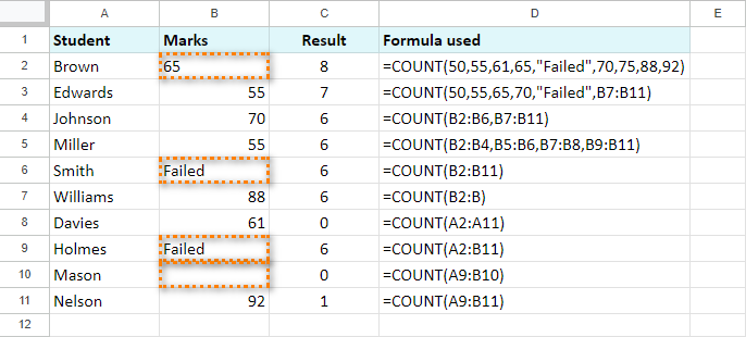
Look, there are different formulas with COUNT in column C.
Since column A contains surnames, COUNT ignores that whole column. But what about cells B2, B6, B9, and B10? B2 has a number formatted as text; B6 and B9 contain pure text; B10 is completely empty.
Another cell to bring your attention to is B7. It has the following formula:
=COUNT(B2:B)
Notice that the range starts from B2 and includes all other cells of this column. This is a very useful method when you often need to add new data to the column but want to avoid changing the range of the formula every time.
Now, how will Google Sheets COUNTA work with the same data?
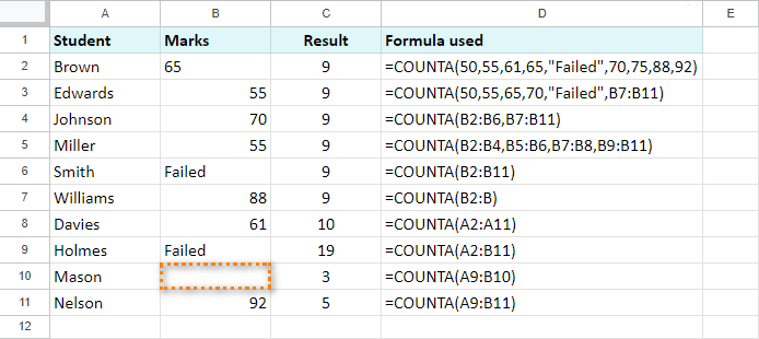
As you can see and compare, the results differ. This function ignores only one cell — the completely empty B10. Thus, bear in mind that COUNTA includes textual values as well as numeric ones.
Here’s another example of using COUNT to find an average sum spent on products:
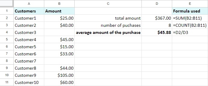
The customers who haven’t bought anything are not considered for the results.
One more peculiar thing regarding COUNT in Google Sheets concerns merged cells. There is a rule that COUNT and COUNTA follow to avoid double counting.
Note. The functions take into account only the leftmost cell of the merged range.
When the range for counting contains merged cells, they will be treated by both functions only if the upper-left cell falls within the counted range.
For example, I merge B6:C6 and B9:C9 and count column B. My formula below will count 65, 55, 70, 55, 81, 88, 61, 92:
=COUNT(B2:B)
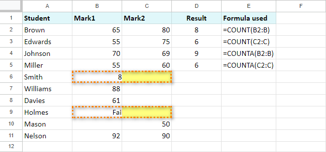
But with a slightly different range, the formula returns another result. It will work only with 80, 75, 69, 60, 50, 90:
=COUNT(C2:C)
The left parts of the merged cells are excluded from this range, therefore are not considered by COUNT.
COUNTA works in a similar way.
=COUNTA(B2:B)counts the following: 65, 55, 70, 55, 81, 88, 61, “Failed”, 92. Just like with COUNT, empty B10 is ignored.=COUNTA(C2:C)works with 80, 75, 69, 60, 50, 90. Empty C7 and C8, as in the case with COUNT, are ignored. C6 and C9 are omitted from the result since the range doesn’t include the leftmost cells B6 and B9.